For my last painting Fun in Djerba, I needed a background with water
Making Fun in Djerba had me experiment a few techniques though, that I thought might be interesting to share.
Pseudo-brownian motion
During my recent collaboration, Portraits n°1 with physicist Ludovic Bellon (read full article here), I came up with a way to energize particles into a Brownian motion. As I don’t exactly follow the strict theoretical rules by considering that my particles can have an acceleration, I was free to define my own version of a noisy force that ends up moving particles in random directions.
\vec{acc} = amp \cdot \vec{dir} \newline \vec{speed} \hspace{2 mm} += \hspace{1 mm} \vec{acc} \newline \vec{speed} \hspace{2 mm} *= \hspace{1 mm} viscosity \newline \vec{x} \hspace{2 mm} += frameDelta \cdot \vec{speed}where the acceleration direction is a random value between 0 and 2 π , the acceleration amplitude is also randomly chosen within a certain range, and viscosity is my simplified version of it, adjusted between 0 and 1.
With this pseudo-Brownian equation that has a random amplitude and direction, the overall result can be quite organic, once you add a blurring layer. Here below is a photoshopped image that shows the raw version of a pseudo-brownian particle background, and a transition to a blurred effect. Surprisingly simple though!
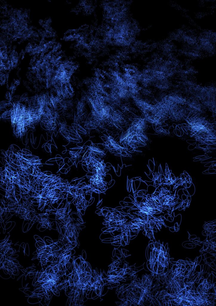
The truth is for this image above I tied a new particle to our moving pseudo-Brownian attractor with a spring force, what we see is the trajectories of such particles, hence the seemingly smooth and circular overall motion.
Modes, size and opacity
Based on those findings, I kept exploring.
Even after adding more particles, with different sizes and colors, I could not quite converge on anything satisfactory. Dang.
Taking a break on the balcony, looking a the water surface of the vibrant blue swimming pool without really paying attention…
Bam!
Modes.
There is a spatial pattern in those wavelets, a characteristic dimension. It’s not a mess, like a white noise, there is some inner order.
So I tried to apply a random mode between 1 and 10 to each particle, and based on their mode I acted on their drawn properties:
- size: the higher the mode, the bigger the dot
- opacity: the higher the mode, the lower the opacity
This means tiny dots are drawn with a sharp opaque brush – relatively opaque, we’re talking 5% maximum because we use many particles – and bigger dots are more blurry.
let a1 = 0.04, a2 = 0.001, // The smaller the neater
    m1 = 1, m2 = this.maxMode

a = a1 + (a2 - a1) * (particle.mode - m1) / (m2 - m1)
The equation above (code language ES6) is just a decreasing linear function where A is the alpha channel in HSLA color space – a variable for opacity/transparency – and m stands for mode.
You instantly get a feeling of depth, like the focus of a camera. At first it felt like the closest particles were rain droplets painted on a window with heavier rain in the background!
This was because between mode 1 and mode 2 the radius was doubled (I had other values of a1 and a2 than those written in the previous code), and only a few particles had mode 1, so the ‘mode 1 layer’ was overly predominant.
By changing the law to something still linear but less violent in terms of scale, it looked nicer.
r = 1.5 * (1 + p.mode/2) * this.dataToImageRatioAlso, I arranged that 50% of all particles have mode 1.
let mode = Math.random() > 0.5 ? 1 : 1 + Math.ceil((this.maxMode - 1) * Math.random())Last but not least, in my previous definition of the pseudo-Brownian noise, I chose a random module for the acceleration vector.
let brownianAngle = 2 * Math.PI * Math.random()
let brownianModule = 10 * p.mode * Math.random()
let xAcc = brownianModule * Math.cos(brownianAngle)
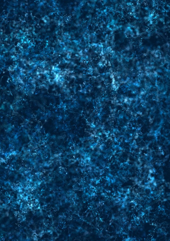
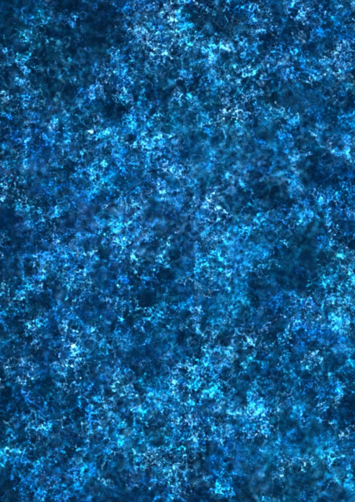
let yAcc = brownianModule * Math.sin(brownianAngle)This means all the values between 0 and the maximum can be set. Removing the random factor cleared all the background from small-scale displacements of bigger particles. As a consequence, nice organic patterns emerged after only a few computational steps!
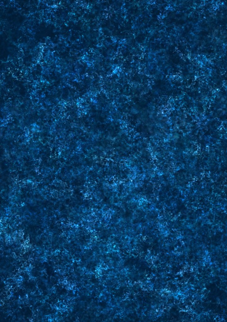
Applying some Speed Light Factor (article), gives the water a subtle motion effect in a certain direction.
To the final artwork
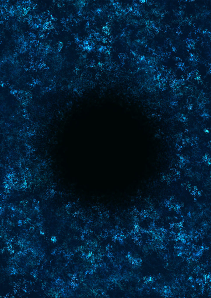
You might have noticed the black hole on the artwork.
This was done with superimposition of two canvases, the one with the water background, and the one with the hole.
The hole is made of dots with radially decreasing sizes.
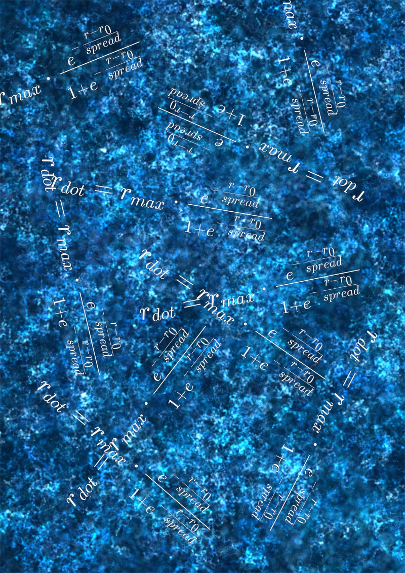
To get control over the hole dimension and its sharpness, I used the very handy following function for transitions:
With the final water background and hole, I could piece the final piece.
Conclude-sion
Despite this article being a bit less detailed than my previous article on a creative process that led me to Djerba Sunset Phoenix, I have explained how I came to play with pseudo-Brownian modes with a goal: painting water with particles.
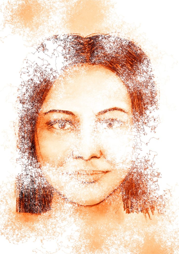
This was a first adventure with water and there is much room for improvement. With this new recipe for organic patterns with particles, I have been able to work on richer background gradients, or re-draw pictures with force field information and particles Browian-wandering around.
Alright folks thanks a lot for reading!